
Reorder an unstructured point cloud into a regular grid, so that neighbor-based operations become simple grid processing.
import gridpoints as grid
points = your_dataset(100000,3) #standard (N, D) array
order = grid.argsort(points, gridshape=(100, 100, 100))  #set gridshape: (I,J,K) = (100,100,100)
Pgrid = points[order].reshape(100, 100, 100, 3)   # now a (I, J, K, D) version of your dataset.
#Ready for convolution, neighbor look-ups or geometrical analysis.
Gridpoints support NumPy, PyTorch and CuPy arrays.
The argsort reordering operation is a one-to-one assignment of your points to cells of a grid with the given gridshape. This is related to Monge optimal transport, but argsort() trades optimality for scalability, by combining greedy axial operations which exploit the specific structure of grids. 1 million 2D/3D points are sorted in about 0.5 s on a GPU (PyTorch) or 10 s on a CPU (NumPy).
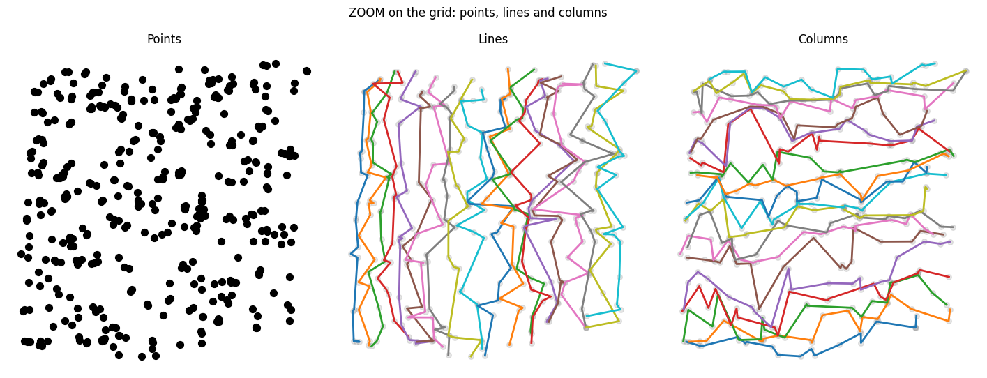
- Problem: point clouds are stored as a flat list
[P1, ..., PN]. Finding the neighbors of a point usually needs a tree or a graph (KD-tree, radius graph...), which is hard to use with standard tensor based machine learning, especially on GPU. - Idea: assign every point to a cell of a D-dimensional grid, one point per cell, such that the grid is sorted along each of its axes. Then the neighbors of a point are approximately the points in nearby cells, found by plain indexing.
- Payoff: local operations (convolution, smoothing, clustering, interpolation...) that are usually hard to implement on irregular point clouds, can be applyed on the grid:
points -> grid. To recover the result on the points, one just apply the invert assignement:grid -> points. - Catch: grid neighborhoods are approximate, not exact (see Limits). It apply in low dimension only <= 7D/8D.
Points are almost always stored in a one-dimensional order. You would like points that are close in space to also be close in memory, so that the nearest neighbor of P[n] is often P[n±1], P[n±2], or a bit further. This is a well-studied problem, and space-filling curves such as the Morton curve are a common solution.
Gridpoints takes a different route. Instead of a 1D order, it gives each point a multi-index [i, j, ...] in a D-dimensional grid. This matters because a grid supports stencil operations: "look at the cells within a few steps in each direction" [i±di, j±dj, k±dk], which is how images and volumes are processed.
Input: a point cloud P of shape (N, D) and a target grid shape (I, J, ...).
Output: a permutation order of the indices such that
Pgrid = P[order].reshape(I, J, ..., D)is a bijection between points and grid cells (one point, one cell), and is sorted along every axis. In 3D, with xyz notation P = (x, y, z):
x[i+1, j, k] >= x[i, j, k]     # x increases along axis 0
y[i, j+1, k] >= y[i, j, k]     # y increases along axis 1
z[i, j, k+1] >= z[i, j, k]     # z increases along axis 2
This property (grid monotonicity) is the only thing guaranteed. See Neighborhood radius for what it does and does not imply.
On Pgrid, a neighbor query becomes a stencil lookup:
neighborhood(Pgrid[i, j, k]) ≈ { Pgrid[i±di, j±dj, k±dk] : (di, dj, dk) within radius R }
where R is a cutoff you choose for your task. Operations built on this run in O(N) on the grid view, instead of relying on graph or tree methods.
pip install gridpoints          # core only
pip install gridpoints[demo]    # adds what the demo notebook needs
Full demo: notebook.ipynb
import gridpoints as grid
import numpy as np

N = 1_000_000
A = np.random.rand(N, 3)                       # raw point cloud (NumPy, PyTorch or CuPy)

# 1. Compute the permutation and view the points as a grid
order = grid.argsort(A, gridshape=(100, 100, 100))
Bflat = A[order]                               # sorted, flat (C-order)
Bgrid = Bflat.reshape(100, 100, 100, 3)        # grid view

# 2. Work on the grid
Cgrid = apply_something(Bgrid)                 # e.g. a convolution; shape (100, 100, 100, *)

# 3. Go back to the original point order
Cflat = Cgrid.reshape(N, -1)
orderinv = grid.invert_permutation(order)
C = Cflat[orderinv]                            # row n corresponds to the original point n
apply_something stands for whatever you want to compute on the grid.
gridpoints.sort() is also available (see the eggshell example below).
The grid shape must be roughly tuned to the kind of data, with the constraint that the number of points N have to be factorised as I⋅J⋅K⋅…
- The exact factorization hardly matters:
(18, 20, 16)and(16, 15, 24)behave similarly. - The orders of magnitude of each dimension matter a lot:
(18, 20, 16)and(36, 40, 4)can give substantially different results. - For a thin surface (e.g. an eggshell), use a flat grid such as
(128, 128, 2). A naive(32, 32, 32)grid on the same data produces a poor representation of the geometry.
Padding : If the number of cells I⋅J⋅K⋅… exceeds the number of points N, the point cloud can be padded with special values (see Padding). This lets you sort a prime or variable number of points, and solves integer-factorization constraints on the grid shape.
Another option to reduce topology-specific effects is to randomly project the data onto one or many lower-dimensional subspace before sorting. Random projections approximately preserve pairwise distances (Johnson–Lindenstrauss lemma).
There is no theoretical guarantee on the radius R needed for a given task. Nearest neighbors are not guaranteed to land in exactly adjacent cells.
Empirically, in 2D, R = 5 captures about 99% of nearest neighbors. Some outliers might sit further away, mostly on complex geometries with sharp peaks, holes or other non-smooth features.
If you need stricter neighborhoods, or work in higher dimension, two options:
- Ensemble of grids: build several grids, each on a rotated or projected view of the points, and combine them (see this discussion).
- Tiling: split the grid into tiles, attach metadata to each tile (e.g. a bounding box), and skip pairs of tiles that are certifiably too far apart for your criterion.
NaN and Inf values are supported in a consistent way by the package, so that padding is natural:
NaN→ placed at a random position±Inf→ placed on the border of the grid
This allow to complete the true N points with ΔN fictive points to match the nearest integer factorisation N + ΔN = IJK…
Sorting 1 million points (2D/3D), measured on a Google Colab T4 GPU:
| Backend | Time |
|---|---|
| NumPy | ~10 s |
| PyTorch (GPU) | ~500 ms |
| CuPy (GPU) | ~1 s (the first, cold call takes ~10 s because of compilation) |
A typical use looks like:
output(i, j, k) = f( Pgrid[i±di, j±dj, k±dk] ) for (di, dj, dk) in a local window
To compute this kind of kernel efficiently, don't use pure python loops which are known to be slow but rather:
- Native grid convolutions of standard libraries, whenever your operation can be expressed that way.
pystencilsortaichifor complex or non-linear kernels.- On GPU, tiling the grid with a custom
tritonkernel can be particularly efficient.
Good fit
- 2D and 3D point clouds, with enough points for O(N) grid operations to pay off.
- Datasets that go beyond smooth, convex blobs: a map of Indonesia, a sponge, a donut, an elephant, an eggshell (with a suitable grid shape). Examples are in the plots folder.
- Pipelines that benefit from regular arrays: GPU processing, convolutions, repeated local operations.
Poor fit
- High dimension. Arbitrary dimension is supported, but the sweet spot is 2D/3D. Dimensions 4 to 6 are still reasonable. Above ~8D, gridpoints is generally not appropriate.
- Small point clouds. Below a few hundred points, the overhead is not worth it: a naive quadratic implementation of your kernels will be simpler and probably faster.
- Geometries that a grid represents badly, e.g. a spider web or a wind turbine. The sort still works, but the resulting grid is a poor representation of the shape. The same applies to a good geometry with a badly chosen grid shape (the eggshell example above).
- Exact neighbors. Neighborhoods are approximate; see Neighborhood radius.
Try it if you process 2D/3D point clouds with local operations, you want regular array layouts (especially on GPU), and approximate neighborhoods are acceptable.
Stay with a KD-tree or a graph method if you need exact nearest neighbors, work in high dimension, or have only a few hundred points.
A quick way to decide is to run the demo notebook on a sample of your own data and check how much of your true nearest neighbors fall within your radius R.